Problem statement
A server exposes an API on the Internet, serving requests. A request has a certain IP as origin. The question is: how should one configure limits on the web server to avoid abusive requests? 'Abusive requests' are a series of requests that happen in bursts of a 'high rate' per second. Nginx allows one to limit request rates. See http://nginx.org/en/docs/http/ngx_http_limit_req_module.html . Above the threshold, Nginx responds with HTTP error 503.
General approach
The general approach is to load web server log data and to measure the request rates from it. After tabulating the data, we can decide what rates are 'abusive'. We'll configure Nginx with
limit_req_zone $binary_remote_addr
meaning that it will apply the request rate limit to the source IP.
Tools
We'll use some Unix commands to pre-process the log files. If you are using Windows, consider installing Cygwin. See https://cygwin.com/install.html .
For R, we can use either a Jupyter notebook or R Studio. Jupyter was useful to organize the commands in sequence, while R Studio was useful to try ad-hoc commands on the data. Both Jupyter notebooks and R Studio are included in Anaconda Navigator. Begin with the "Miniconda" install. See https://conda.io/miniconda.html .

Install R Studio and Jupyter notebook from Anaconda Navigator.
Pre-processing the web server logs
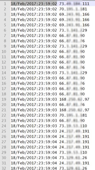
The log files have lines including many information. We just need the date+time and source IP.

We cut twice, first on double-quotes, then on whitespace. Then we remove some extra characters if needed.
cut -d "\"" -f1,8 fdpapi_ssl_access_w2_21.log | cut -d " " -f4,6 | sed 's/\[//' | sed 's/,//' | sed 's/\"//' > fdpapi_ssl_access_w2_21.csv The end result are lines with just the date+time and source IP.
Analysing the logs
The first lines of the R script load the csv file. Then, sort the rows by IP.
library(readr)
logrows <- read_delim("~/TGIF_work/nginx_thr_FDPCARE-325/fdpapi_ssl_access_w_tutti.csv",
" ", escape_double = FALSE, col_names = FALSE,
col_types = cols(`coldatetime` = col_datetime(format = "%d/%b/%Y:%H:%M:%S"),
X1 = col_datetime(format = "%d/%b/%Y:%H:%M:%S")),
trim_ws = TRUE)
logrows <- logrows[order(logrows$X2),]
You can peek into the log rows.
head(logrows)
| X1 | X2 |
|---|---|
| 2017-02-19 00:00:04 | 100.0.XX.244 |
| 2017-02-19 00:00:04 | 100.0.XX.244 |
| 2017-02-19 00:03:51 | 100.1.XXX.223 |
| 2017-02-19 00:03:51 | 100.1.XXX.223 |
| 2017-02-19 00:03:52 | 100.1.XXX.223 |
| 2017-02-19 00:02:48 | 100.1.XXX.60 |
R has a special type called 'factor' to represent unique 'categories' in the data. Each element in the factor is called a 'level'. In our case, unique IPs are levels.
tb <- table(logrows$X2) ipsfactor <- factor(logrows$X2, levels = names(tb[order(tb, decreasing = TRUE)]))
Let us define a function to translate the request times into numbers (minutes) relative to the first request. Then, make a histogram of the requests, placing them into 'bins' of one minute.
# x is a vector with the datetimes for a certain IP findfreq <- function(x) {
thesequence <- as.numeric(x-min(x), units="mins")
hist(thesequence, breaks = seq(from = 0, to = ceiling(max(thesequence))+1, by=1), plot=FALSE)$counts
}
Here we could count the frequency of IPs using the factor and the function. That is, we could apply the function for each IP. This would allow for the visualization of an 'intermediary' step of the process.
# Intermediary steps # ipscount <- tapply(logrows$X1, ipsfactor, findfreq, simplify=FALSE)
# ttipscount <- t(t(ipscount))
Transposing the array twice simplifies the visualization.
Let's now define another similar function that only keeps the maximum.
findmaxfreq <- function(x) {
max(findfreq(x))
}
Aggregate the data using the new function.
ipsagg <- aggregate( logrows$X1 ~ ipsfactor, FUN = findmaxfreq )
Display the top IPs sorted by requests per minute descending. These are the 'top abusers'. The table shows that IP 51.XXX.56.29 sent 1160 requests per minute at one point.
head(ipsagg[order(ipsagg$`logrows$X1`, decreasing = TRUE),]) | ipsfactor | logrows$X1 |
|---|---|
| 51.XXX.56.29 | 1160 |
| 64.XX.231.130 | 711 |
| 64.XX.231.169 | 705 |
| 68.XX.69.191 | 500 |
| 217.XXX.203.205 | 462 |
| 64.XX.231.157 | 458 |
Display quantiles from 80% to 100%
quantile(ipsagg$`logrows$X1`, seq(from=0.99, to=1, by=0.001)) 
This table is saying that 99.6% of the IPs had the max request rate of 63 requests per minute or less. Plot the quantiles.
ipsaggrpm <- ipsagg$`logrows$X1`
n <- length(ipsaggrpm)
plot((1:n - 1)/(n - 1), sort(ipsaggrpm), type="l",
main = "Quantiles for requests per minute",
xlab = "Quantile fraction",
ylab = "Requests per minute")

As you can see in the quantiles table and the graph, there is a small percentage of 'abusive' source IPs.
Web server request limit configuration
Fron Nginx documentation: " If the requests rate exceeds the rate configured for a zone, their processing is delayed such that requests are processed at a defined rate. Excessive requests are delayed until their number exceeds the maximum burst size in which case the request is terminated with an error 503 (Service Temporarily Unavailable). By default, the maximum burst size is equal to zero. ". In this sample case, considering that 99.6% of the IPs issued 63 requests per minute or less, considering each source IP, we can set the configuration as follows:
limit_req_zone $binary_remote_addr zone=one:10m rate=63r/m;
...
limit_req zone=one burst=21;
And burst is set to one-third of 63 requests per minute. This is considering one web server. If a Load Balancer is forwarding requests evenly to two servers, consider half of the values above:
limit_req_zone $binary_remote_addr zone=one:10m rate=32r/m;
...
limit_req zone=one burst=11;
Useful links
Matrix Operations in R
Dates and Times in R
Dates and Times Made Easy with lubridate - I didn't have to use lubridate, but I "almost" did.
Quantiles
Download the Jupyter notebook with the R script
You can download the Jupyter notebook with the R script here: https://1drv.ms/u/s!ArIEov4TZ9NM_HBIav7QiNR28Gmu .